The time-delay neural betwork (TDNN) is widely used in speech recognition software for the acoustic model, which converts the acoustic signal into a phonetic representation. The papers describing the TDNN can be a bit dense, but since I spent some time during my master’s thesis working with them, I’d like to take a moment to try to demystify them a little.

Actually, if you are already familiar with neural networks, then here’s the big spoiler:

The TDNN is essentially a 1-d convolutional neural network without pooling and with dilations.

That’s a mouthful, so the rest of this blog post is going to introduce the arithmetic of what that actually means.

By the way, in terms of CNNs in general, the mathematics are well described in [1] and [2], the latter from which I have lifted/edited some code to generate the images in this post.

$ \definecolor{tdnn01}{RGB}{55, 70, 171} \definecolor{tdnn02}{RGB}{120, 81, 156} \definecolor{tdnn03}{RGB}{189, 93, 194} \definecolor{tdnncyan}{RGB}{42,161,152} $

The TDNN was originally designed by Waibel ([4], [5]) and later popularized by Peddinti et al ([3]), who used it as part of an acoustic model. It is still widely used for acoustic models in modern speech recognition software (such as Kaldi) in order to convert an acoustic speech signal into a sequence of phonetic units (phones).

The inputs to the network are the frames of acoustic features. The outputs of the TDNN are a probability distribution over each of the phones defined for the target language. That is, the goal is to read the audio one frame at a time, and to classify each frame into the most likely phone.

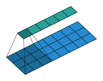
In one layer of the TDNN, each input frame is a column vector representing a single time step in the signal, with the rows representing the feature values. The network uses a smaller matrix of weights (the kernel or filter), which slides over this signal and transforms it into an output using the convolution operation, which we will see in a moment.

We can visualize the kernel (dark blue area) moving over the input (light blue) to produce the output (green) like so:

Mathematically, let’s assume that we have an input vector $\mathbf{x_t} \in \mathbb{R}^m$ with some numbers in it, such as the amplitudes at a given frequency, or the values in a filter bank bin. We collect these vectors into a matrix, where each vector represents one time step $t$ of our speech signal e.g. one sample taken every 10 miliseconds. (The visualization of this matrix is often called a spectrogram.)

Observing the input over time, we then have the matrix of input features $\mathbf{X} \in \mathbb{R}^{m \times t}$.

Let us also define a trainable weight matrix (the kernel or filter) $\mathbf{W} \in \mathbb{R}^{m \times l}$, where the kernel has the same height of $m$, and a width of $l$. So visually, it would look a little like this:

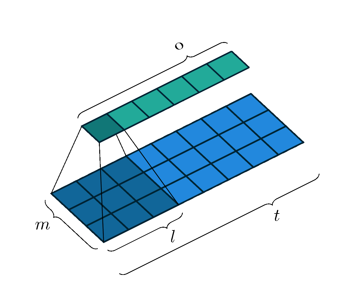
The kernel $\mathbf{W}$ slides over the input signal, with a stride of $s$, so it makes $s$ steps at a time. The region on the input feature map that the kernel covers is called the receptive field. Depending on the implementation, the input could be padded with null values of padding of height $m$ and length $p$ on either end. For simplicity, let’s assume we have no padding ($p=0$), and that the kernel slides over the input signal one step at a time ($s=1$). This is a typical scenario, and also the one that I have illustrated in the images.

Moving in this way, the output width $o$, that is, the number of times that the kernel can “fit” across the length of the input sequence, is given by:

\begin{equation} o = \left\lfloor\dfrac{t-l+2p}{s} \right\rfloor + 1 \label{eq:tdnn-neuron-output-size} \end{equation}

where $\lfloor . \rfloor$ indicates the floor function.

At each time step $t$, the TDNN performs a convolution operation, which is an operation that takes an element-wise multiplication (Hadamard product) of the kernel weights over the input beneath it, and sums those multiples together. In the neural network, a trainable bias $b$ is added (not pictured in the images above), and the result is passed through a non-linear activation function $\phi$ (e.g. sigmoid as in [4], rectified linear, or $p$-norm as in [3]) to form the output $z_q \in \mathbf{z}$, where $\mathbf{z}$ is the entire output vector after doing this operation for all the time steps (the light green vector in the images).

So, the scalar output of a single element $z_q \in \mathbf{z}$, at output step $q \in \{1,2,…,o\}$, can be succinctly given by:

\begin{equation} z_q = \phi(\mathbf{W} * \mathbf{X_{q}} + \mathbf{b}) \end{equation}

where $*$ denotes the convolution operation and $\mathbf{X_{q}}$ are the inputs in the receptive field.

It can also be equivalently given by:

\begin{equation} z_q = \phi ( { \color{tdnn01} \sum_{i=1}^{m} } { \color{tdnn02} \sum_{k=1}^{l} } w_{i,k} \ x_{i,k} + b) \label{eq:tdnn-summation} \end{equation}

where the first summation ranges over the height of the acoustic features, the second over the width of the receptive field/width of the kernel.

Note that the kernel weights (the $w_{i,k}$) are shared for each output step $q$. Because the kernel’s weights are shared across the convolutions, the TDNN learns a representation of the input that is invariant to the specific position of a phone in the larger sequence. This also cuts down on the number of parameters we have to train. It’s a win-win.

For a more complicated case, the kernel may not pass over contiguous feature vectors. That is, the input to the kernel may be the current frame, plus some frame a little while in the past and some frame a little while in the future. The past/future frames are often referred to as the “context” or as the “delays,” and the process of looking at non-contiguous frames like this can also be referred to as “dilation” or “subsampling” in the literature.

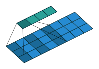
In this case, the summation will occur over only those values directly beneath the kernel, which now has some gaps in its length. Thus, we can define $J$ as the set of context frame indexes to select, with $j=0$ as the time step currently being processed. Example $J$s may be, e.g. the range of integers $[-2,2]$ or the set of integers $\{-7,0,1\}$.

The size of the output vector (i.e. the number of times the kernel can “fit” into the input space) will be defined by the range of the values in $J$ as follows:

\begin{equation} o = \left\lfloor\dfrac{t-(\text{max}(J)-\text{min}(J))+2p}{s} \right\rfloor \label{eq:tdnn-neuron-output-size-subsampled} \end{equation}

This corresponds to the following image:

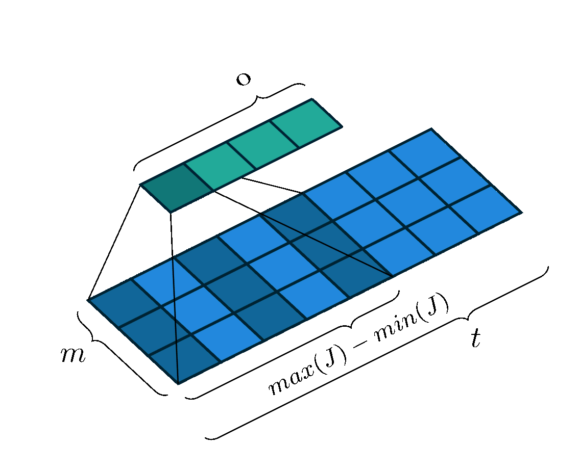
Mathematically, we still perform the same convolution operation as before $z_q = \phi(\mathbf{W} * \mathbf{X_{q}} + \mathbf{b})$; however, the input vectors $\mathbf{X_{q}}$ have now changed, because the receptive field has changed. Intuitively, we can think of the operation as extracting the receptive field from its input, glueing it together, and performing the same convolution operation.

Finally, let us suppose that instead of just one kernel, we have $H$ kernels, such that $\mathbf{W^{(h)}} \in {\mathbf{W^{(1)}}, …, \mathbf{W^{(H)}}}$. Each kernel can be used to similarly slide over the input. This will create a series of output vectors, which we can organize into an output matrix $\mathbf{Z} \in \mathbb{R}^{h \times o}$.

In a deep neural network architecture, this output can then become the first hidden layer of the network, and be used as input to the next layer of the TDNN. An example with two hidden layers is illustrated in its full glory in [4]:

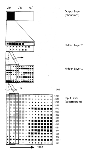
In this image, we see a contiguous TDNN (no dilations). We can see that receptive field for the first hidden layer covers three frames of the input feature map on the interval $[-1,1]$ (i.e. a total of $3$ frames: the target and $\pm 1$ frames), and it is convolved with $8$ kernels to create the first hidden layer. A stride of $1$ is used to pass over the entire input signal. Then, frames on the interval $[-2,2]$ (i.e. a total of $5$ frames) are convolved with $3$ kernels to produce the second hidden layer. In the original paper, the rows from the second layer are then summed to produce the output distribution over the $3$ output phone classes.

As a side note, to perform the convolution as a matrix operation, the input and kernel can be unrolled, and a dot product can be computed. That is, let’s say we have an example input matrix and kernel matrix like so:

\begin{equation} \mathbf{X} = \begin{bmatrix} x_{1,1} & x_{1,2} & x_{1,3} & x_{1,4} \\ x_{2,1} & x_{2,2} & x_{2,3} & x_{2,4} \\ x_{3,1} & x_{3,2} & x_{3,3} & x_{3,4} \end{bmatrix} \end{equation}

\begin{equation} \mathbf{W} = \begin{bmatrix} w_{1,1} & w_{1,2} \\ w_{2,1} & w_{2,2} \\ w_{3,1} & w_{3,2} \end{bmatrix} \end{equation}

When we unroll the input, we just concatenate the rows together into a single vector.

We then create a new sparse matrix for the kernel of size $o \times n$, where $o$ is the number of output steps as described above and $n$ is the length of the unrolled input vector. The entries in each row are the weights, where needed, or $0$s elsewhere (a Toeplitz matrix).

We can now take the dot product with the inputs like so:

\begin{equation} \begin{bmatrix} w_{1,1} & w_{1,2} & 0 & 0 & w_{2,1} & w_{2,2} & 0 & 0 & w_{3,1} & w_{3,2} & 0 & 0 \\ 0 & w_{1,1} & w_{1,2} & 0 & 0 & w_{2,1} & w_{2,2} & 0 & 0 & w_{3,1} & w_{3,2} & 0 \\ 0 & 0 & w_{1,1} & w_{1,2} & 0 & 0 & w_{2,1} & w_{2,2} & 0 & 0 & w_{3,1} & w_{3,2}
\end{bmatrix} \cdot \begin{bmatrix} x_{1,1} \\ x_{1,2} \\ x_{1,3} \\ x_{1,4} \\ x_{2,1} \\ x_{2,2} \\ x_{2,3} \\ x_{2,4} \\ x_{3,1} \\ x_{3,2} \\ x_{3,3} \\ x_{3,4} \\ \end{bmatrix} \end{equation}

In terms of training the neural network, we use the typical backpropagation algorithm of neural networks. Once we have the loss, we multiply it with the transpose of the sparse weights matrix to make the updates.

The TDNN works well for speech recognition, because we are able to take advantage of the temporal nature of the acoustic signal by varying the context in each hidden layer. We can skip over frames very close to our target frame, which are likely very similar to our target frame (e.g. they represent the same phone), and instead look at context frames a little further out. This allows us to convert a very dense acoustic signal into a more abstract phonetic representation.

If you want to learn more about the TDNN (and its big brother, the CNN), I recommend checking out the references I’ve mentioned below, which can do this topic better justice: [1] and [2] cover the arithmetic of convolutional neural networks in general, and provide some great visualizations, while [3], [4], and [5] are the original papers that deal with the TDNN specifically.

References

[1] Karpathy, A. CS231n: Convolutional Neural Networks for Vision Recognition. http://cs231n.github.io/convolutional-networks/

[2] Dumoulin, V. and Visin, F. (2016). A guide to convolution arithmetic for deep learning. arXiv preprint arXiv:1603.07285. https://arxiv.org/pdf/1603.07285.pdf and https://github.com/vdumoulin/conv_arithmetic

[3] Peddinti, V., Povey, D., and Khudanpur, S. (2015). A time delay neural network architecture for efficient modeling of long temporal contexts. In Sixteenth Annual Conference of the International Speech Communication Association. https://www.isca-speech.org/archive/interspeech_2015/papers/i15_3214.pdf

[4] Waibel, A., Hanazawa, T., Hinton, G., Shikano, K., and Lang, K. J. (1990). Phoneme recognition using time-delay neural networks. In Readings in speech recognition, pages 393–404. Elsevier. https://www.cs.toronto.edu/~hinton/absps/waibelTDNN.pdf

[5] Waibel, A. (1989). Modular construction of time-delay neural networks for speech recognition. Neural computation, 1(1):39–46. https://ieeexplore.ieee.org/document/6795666

Cite This Blog Post

Tchistiakova, S. (2019). Time Delay Neural Network. https://kaleidoescape.github.io/tdnn

@misc{tchistiakova_2019, 
  title={Time Delay Neural Network},
  url={https://kaleidoescape.github.io/tdnn/}, 
  author={Tchistiakova, Svetlana},
  year={2019},
  month={Nov} 
}